


|
|
|
Data pre-processing | |
|---|
Here, we describe the basic pre-processing steps required for tractography using constrained spherical deconvolution. We will also show how to generate a number of useful additional images and maps, whose use is recommended.
A brain mask image is useful for a number of reasons. First, it can be used to clean up tensor maps by removing noisy voxels outside the brain. Second, it can be used to prevent tracks generated by the fibre-tracking algorithm from propagating outside the head. Last, and most important, it can significantly speed up the CSD computation, by preventing the analysis of non-brain voxels.
For the purposes outlined above, the brain mask should have the same dimensions as the DWI data set. The simplest approach is to extract the b=0 image from the DWI data set (this example assumes that the first volume in the data set is a b=0 volume):
> average dwi.mif -axis 3 - | threshold - - | median3D - - | median3D - mask.mif
average: averaging... 100%
threshold: finding min/max... 100%
threshold: building histogram... 100%
threshold: thresholding at intensity 25.5115... 100%
median3D: median filtering... 100%
median3D: median filtering... 100%
Note: this example uses pipes to execute a chain of commands. These are described in more detail here.
The threshold value is in this case determined using simple histogram binning. You can specify your own threshold if you wish, by supplying the appropriate option to threshold.
While this procedure should produce a reasonable mask of the brain, it is by no means fail-proof. You are strongly encouraged to check the brain mask using MRView. If you need to edit the mask (for example, if some parts of the brain were not included), you can do so using the ROI analysis sidebar tool within MRView.
This section describes the steps necessary to the diffusion tensor and associated parameters (see e.g. Basser & Jones, 2002 for a review). The various tensor maps are generated as follows:
> dwi2tensor dwi.mif dt.mif
dwi2tensor: converting DW images to tensor image... 100%
Note: in case the DWI data set headers do not include the DW scheme, you will need to supply your own encoding file (see here for details). This can be done as follows (assuming encoding.b is the encoding file):
> dwi2tensor dwi.mif -grad encoding.b dt.mif
dwi2tensor: converting DW images to tensor image... 100%
> tensor2FA dt.mif - | mrmult - mask.mif fa.mif
tensor2FA: generating fractional anisotropy map... 100%
mrmult: multiplying... 100%
Note that the FA map generated above has been multiplied by the brain mask image to remove the noisy background.
> tensor2vector dt.mif - | mrmult - fa.mif ev.mif
tensor2vector: generating major eigenvector map... 100%
mrmult: multiplying... 100%
Note that the EV map generated above has been scaled by the FA map.
This section describes the steps necessary to perform constrained spherical deconvolution (for a detailed description of the technique, please refer to Tournier et al.. 2004 and Tournier et al. 2007).
> erode mask.mif -npass 3 - | mrmult fa.mif - - | threshold - -abs 0.7 sf.mif
erode: eroding ... 100%
erode: eroding ... 100%
erode: eroding ... 100%
mrmult: multiplying... 100%
threshold: thresholding at intensity 0.7... 100%
The initial erosion step ensure that no edge voxels with artefactually high FA are included in the single-fibre mask. This mask is then applied to the FA map, and the resulting image is thresholded at FA = 0.7.
Note that this value is a guide only - feel free to use a different value if this does not produce satisfactory results. Ideally, you should now have a mask containing a few hundred voxels, all located within high FA white matter regions. It is very important to check that the single-fibre mask is suitable, as otherwise the response function produced in the following step may be totally inappropriate, which would seriously affect the quality of the CSD output. If needed, you can edit this mask image to remove unwanted voxels using the ROI analysis sidebar tool within MRview.
The response function SH coefficients can now be estimated from the DW signal in the single-fibre voxels:
> estimate_response dwi.mif sf.mif response.txt
estimate_response: estimating response function... 100%
This should produce the text file response.txt, containing a series of numbers, such as:
232.781 -122.139 52.8959 -17.3446 3.53066
Note: use the -grad option to supply your own DW scheme if none is to be found in the DWI data set headers.
Normally, the values in the response file should alternate between positive and negative while decreasing in magnitude. The first value should be positive, and have an amplitude similar to (but not necessarily the same as) the b=0 brain white matter signal (you can verify this by loading the dwi.mif image and placing the focus within a white matter region - the intensity is displaced in the bottom right of the statusbar). Note that this is only an approximate guideline: it is not unusual for the first coefficient to differ from the b=0 signal quite significantly (on the other hand, if they differ by orders of magnitude, something has definitely gone wrong).
You can also use the disp_profile command to display the response function:
> disp_profile -response response.txt
This will open a window with a 3D rendering of the response function:
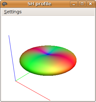
The response function should be broadest in the axial plane, and have low amplitude along the z-axis. If this is not the case, it is likely that the estimate_response program has used a maximum harmonic order that is too high given the data. You can override this value using the -lmax option, for example:
> estimate_response dwi.mif sf.mif -lmax 6 response.txt
estimate_response: estimating response function... 100%
In general, a value of 6 or 8 is adequate (the number provided must be even). As a guide, this number should be chosen such that the number of distinct DW directions used in the acquisition is greater than the number of parameters that need to be estimated. For convenience, a table of the number of parameters required for various maximum harmonic orders is provided below:
| Maximum harmonic order (lmax) | Number of parameters required |
|---|---|
| 2 | 6 |
| 4 | 15 |
| 6 | 28 |
| 8 | 45 |
| 10 | 66 |
| 12 | 91 |
| n | ½ (n+1)(n+2) |
The CSD computation itself can now be performed:
> csdeconv dwi.mif response.txt -lmax 8 -mask mask.mif CSD8.mif
csdeconv: performing constrained spherical deconvolution... 100%
Here, the maximum harmonic order lmax has been set to 8, which should be suitable for most DWI data sets. You may need to alter this value for different acquisition parameters. Also, the brain mask has been used here to prevent unnecessary computations in non-brain voxels; this can speed up the computation time significantly.
On multi-core systems, the computation time can also be reduced significantly using parallel processing. The csdeconv command is capable of running in multi-threaded mode. To use this feature, set the NumberOfThreads parameter in the MRtrix configuration file.
Note: use the -grad option to supply your own DW scheme if none is to be found in the DWI data set headers.Once the processing is done, you can display the results using the orientation plot sidebar tool within MRview.
|
|
|
top | |
|---|